Estimation Explained: How We Guess Population Values from a Sample
September 4 2026 • 3 min read

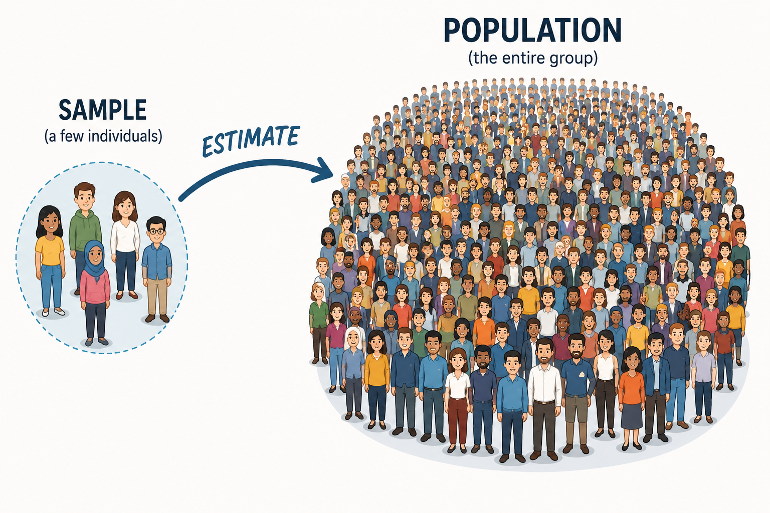
Image by AI
Estimation is one of the two main tools of statistical inference — the process of drawing conclusions about a population based on data collected from a sample. Instead of measuring every single person or item in a population, researchers study a smaller group and use that data to make an educated guess about the whole.
The Problem: We Can't Measure Everyone
Imagine trying to find the average blood pressure of an entire country's population. Measuring every single person is impossible, so instead we measure a sample — say, 30 patients — and use that sample to estimate the true population value.
This is the core idea of inference: we move from a statistic (calculated from the sample) to a parameter (the true, usually unknown, value in the population).
Point Estimation vs. Interval Estimation
There are two ways to present an estimate:
- Point estimate: a single number, such as a mean or a percentage. For example, "average SBP = 120 mmHg."
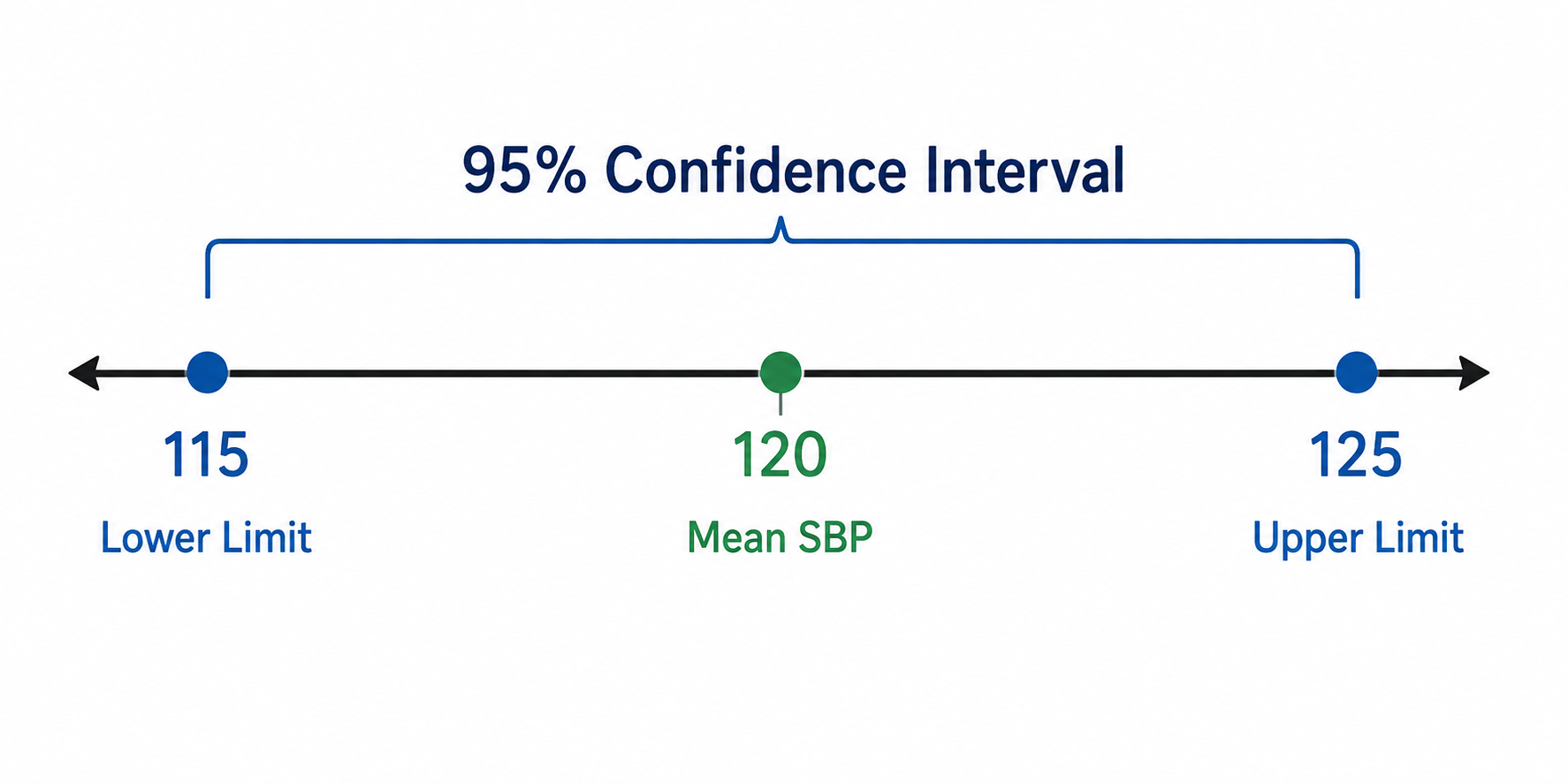
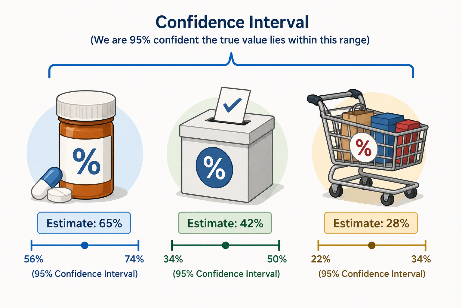
- Interval estimate: a range of values, known as a confidence interval, that is likely to contain the true population value. For example, "average SBP = 120 mmHg (95% CI: 115, 125 mmHg)."
A point estimate alone doesn't tell you how much uncertainty surrounds it. A confidence interval does — it communicates both the best guess and the precision of that guess.

Parameters vs. Estimates
A quick note on notation, since it appears throughout the calculations below:
- Parameter (θ or μ): the true, fixed value in the population — almost always unknown.
- Estimate (θ̂ or x̄): the value calculated from the sample, used to approximate the parameter.
The General Formula for a Confidence Interval
Nearly every confidence interval follows the same basic structure:
Point Estimate ± (Reliability Coefficient × Standard Error)
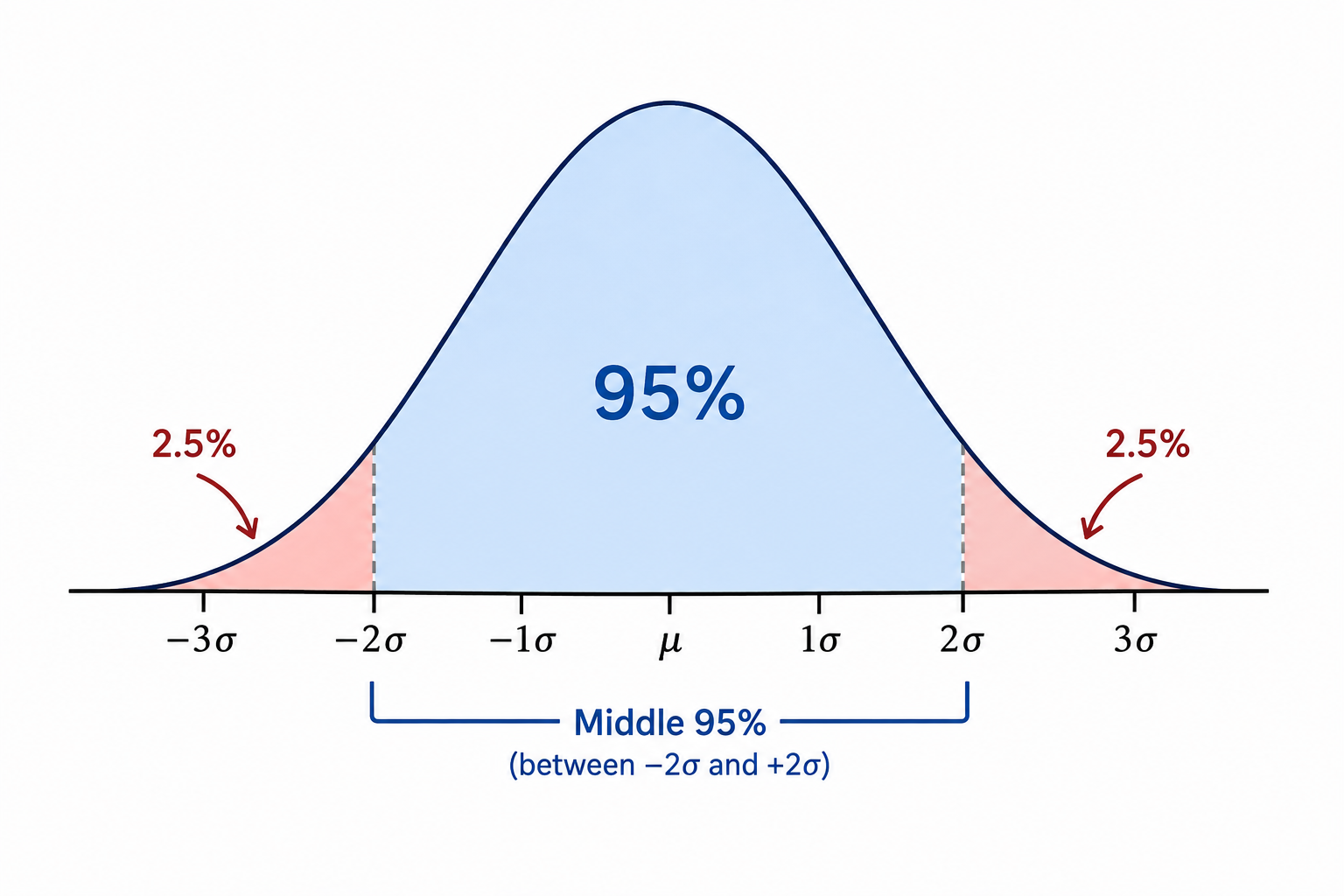
The reliability coefficient depends on how confident you want to be, and comes from the standard normal (z) distribution:
| Confidence Level | Reliability Coefficient (z) |
|---|---|
| 90% | 1.65 |
| 95% | 1.96 |
| 99% | 2.58 |
A higher confidence level requires a larger coefficient, which produces a wider interval — more certainty comes at the cost of precision.
Example: Estimating a Population Mean
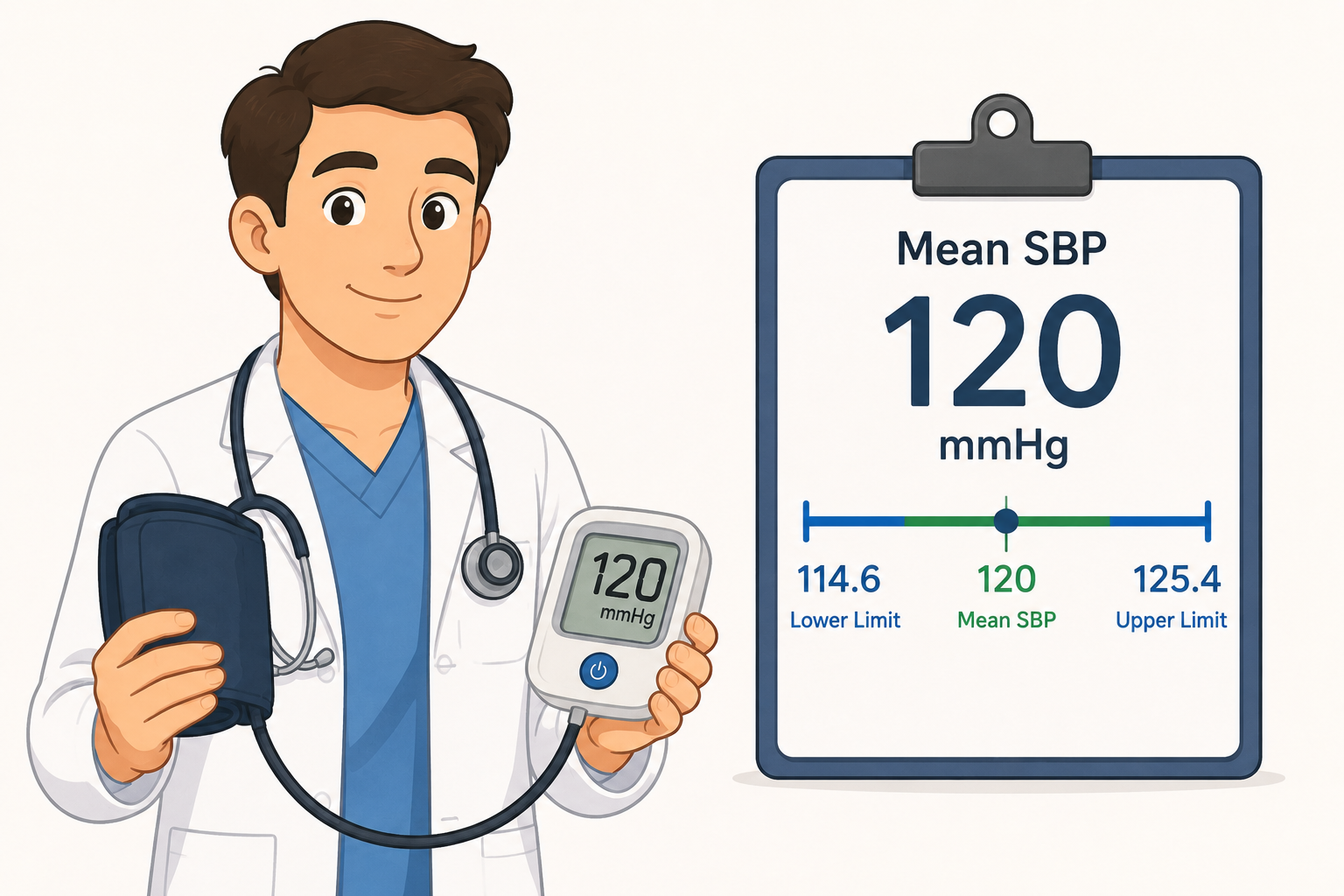
Suppose systolic blood pressure (SBP) was measured in 30 patients, giving a mean of 120 mmHg and a standard deviation of 15 mmHg. To estimate the population mean with 95% confidence:
120 ± 1.96 × (15 / √30)
120 ± 1.96 × 2.739
95% CI: 114.6, 125.4
Interpretation: we are 95% confident that the true population mean SBP lies between 114.6 and 125.4 mmHg.
Example: Estimating a Population Proportion
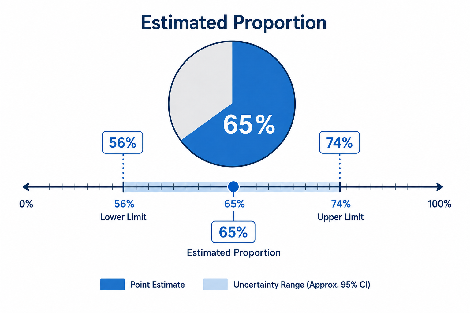
Estimation also applies to proportions or percentages — for example, the proportion of a population with a disease. In a study of drug users, 130 out of 200 tested HIV positive. To estimate the population proportion with 99% confidence:
p̂ = 130/200 = 0.65
0.65 ± 2.58 × √(0.65 × 0.35 / 200)
99% CI: 0.5623, 0.7377
Interpretation: we are 99% confident that the true population percentage of HIV-positive individuals is between 56.23% and 73.77%.
Note: the normal approximation for proportions only works well when both np and n(1-p) are greater than 5.
💡 The Bottom Line
A single number is rarely the whole story. Whenever you report a mean or a proportion from a sample, pair it with a confidence interval so readers know not just your best guess, but how much uncertainty surrounds it.
Report your point estimate. Compute your confidence interval. Interpret with care.